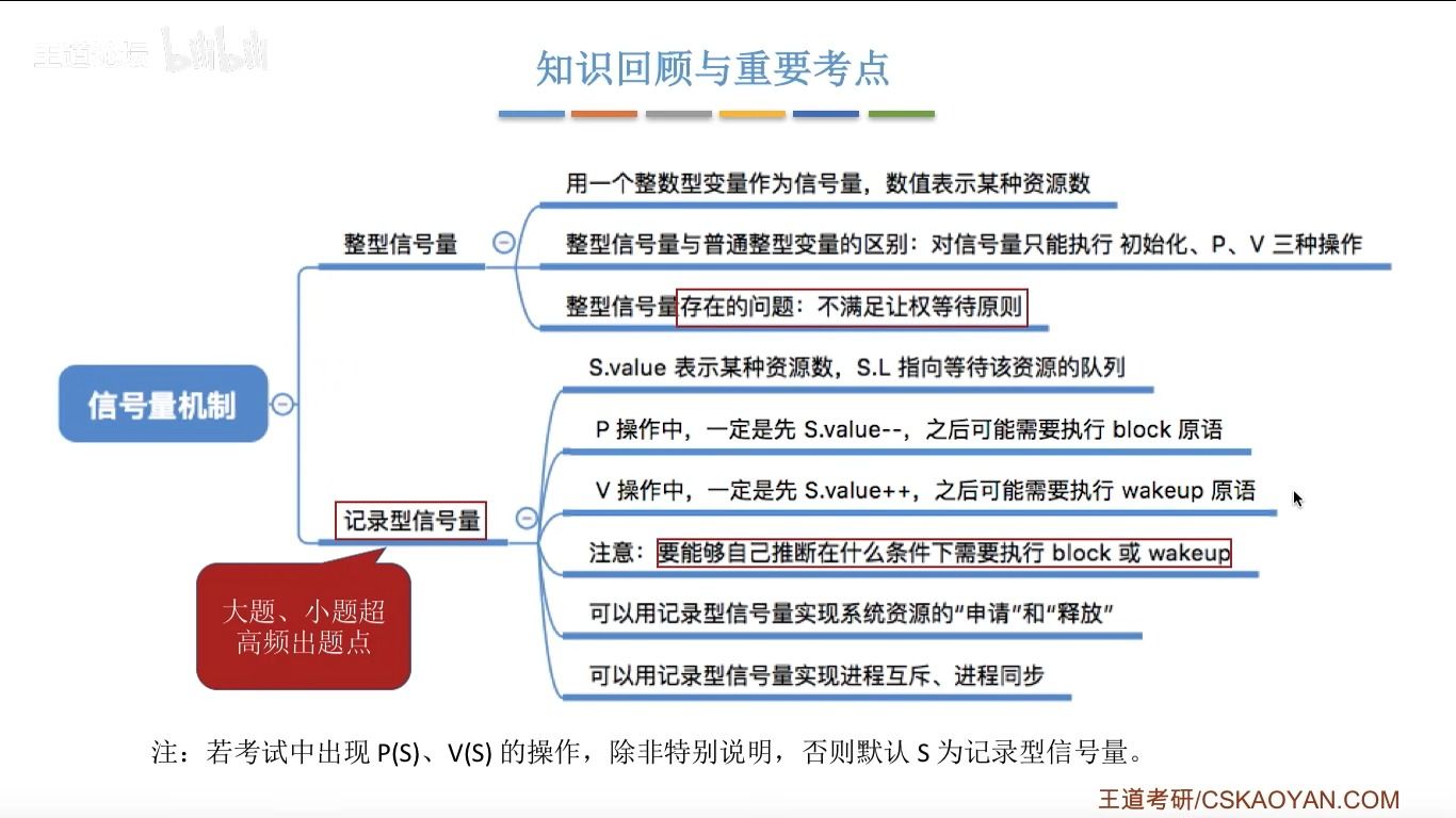
一、显示 API 简介
使用 utils.discovery.all_displays 查找可用的 API。
Sklearn 的
utils.discovery.all_displays可以让你看到哪些类可以使用。
from sklearn.utils.discovery import all_displays
displays = all_displays()
displays
Scikit-learn (sklearn) 总是会在新版本中添加 "Display "API,因此这里可以了解你的版本中有哪些可用的 API 。例如,在我的 Scikit-learn 1.4.0 中,就有这些类:
[('CalibrationDisplay', sklearn.calibration.CalibrationDisplay),
 ('ConfusionMatrixDisplay',
  sklearn.metrics._plot.confusion_matrix.ConfusionMatrixDisplay),
 ('DecisionBoundaryDisplay',
  sklearn.inspection._plot.decision_boundary.DecisionBoundaryDisplay),
 ('DetCurveDisplay', sklearn.metrics._plot.det_curve.DetCurveDisplay),
 ('LearningCurveDisplay', sklearn.model_selection._plot.LearningCurveDisplay),
 ('PartialDependenceDisplay',
  sklearn.inspection._plot.partial_dependence.PartialDependenceDisplay),
 ('PrecisionRecallDisplay',
  sklearn.metrics._plot.precision_recall_curve.PrecisionRecallDisplay),
 ('PredictionErrorDisplay',
  sklearn.metrics._plot.regression.PredictionErrorDisplay),
 ('RocCurveDisplay', sklearn.metrics._plot.roc_curve.RocCurveDisplay),
 ('ValidationCurveDisplay',
  sklearn.model_selection._plot.ValidationCurveDisplay)]
二、显示决策边界
使用 inspection.DecisionBoundaryDisplay 显示决策边界
如果使用 Matplotlib 来绘制,会很麻烦:
使用
np.linspace设置坐标范围;使用
plt.meshgrid计算网格;使用
plt.contourf绘制决策边界填充;然后使用
plt.scatter绘制数据点。现在,使用
inspection.DecisionBoundaryDisplay可以简化这一过程:
from sklearn.inspection import DecisionBoundaryDisplay
from sklearn.datasets import load_iris
from sklearn.svm import SVC
from sklearn.pipeline import make_pipeline
from sklearn.preprocessing import StandardScaler
import matplotlib.pyplot as plt

iris = load_iris(as_frame=True)
X = iris.data[['petal length (cm)', 'petal width (cm)']]
y = iris.target


svc_clf = make_pipeline(StandardScaler(),
                        SVC(kernel='linear', C=1))
svc_clf.fit(X, y)

display = DecisionBoundaryDisplay.from_estimator(svc_clf, X,
                                                 grid_resolution=1000,
                                                 xlabel="Petal length (cm)",
                                                 ylabel="Petal width (cm)")
plt.scatter(X.iloc[:, 0], X.iloc[:, 1], c=y, edgecolors='w')
plt.title("Decision Boundary")
plt.show()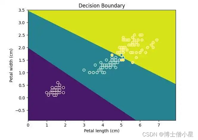
使用 DecisionBoundaryDisplay 绘制三重分类模型。
请记住,
Display只能绘制二维数据,因此请确保数据只有两个特征或更小的维度。
三、概率校准
要比较分类模型,使用 calibration.CalibrationDisplay 进行概率校准,概率校准曲线可以显示模型预测的可信度。
CalibrationDisplay使用的是模型的predict_proba。如果使用支持向量机,需要将probability设为 True:
from sklearn.calibration import CalibrationDisplay
from sklearn.model_selection import train_test_split
from sklearn.datasets import make_classification
from sklearn.ensemble import HistGradientBoostingClassifier

X, y = make_classification(n_samples=1000,
                           n_classes=2, n_features=5,
                           random_state=42)
X_train, X_test, y_train, y_test = train_test_split(X, y,
                                            test_size=0.3, random_state=42)
proba_clf = make_pipeline(StandardScaler(),
                          SVC(kernel="rbf", gamma="auto",
                              C=10, probability=True))
proba_clf.fit(X_train, y_train)

CalibrationDisplay.from_estimator(proba_clf,
                                            X_test, y_test)

hist_clf = HistGradientBoostingClassifier()
hist_clf.fit(X_train, y_train)

ax = plt.gca()
CalibrationDisplay.from_estimator(hist_clf,
                                  X_test, y_test,
                                  ax=ax)
plt.show()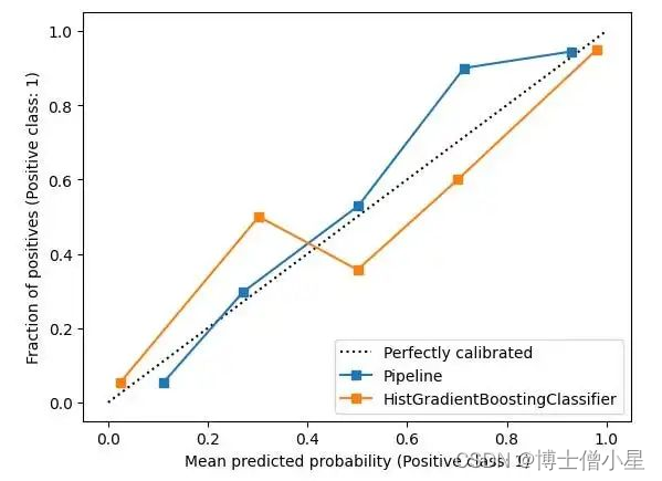
CalibrationDisplay.
四、显示混淆矩阵
在评估分类模型和处理不平衡数据时,需要查看精确度和召回率。使用
metrics.ConfusionMatrixDisplay绘制混淆矩阵(TP、FP、TN 和 FN)。
from sklearn.datasets import fetch_openml
from sklearn.ensemble import RandomForestClassifier
from sklearn.metrics import ConfusionMatrixDisplay

digits = fetch_openml('mnist_784', version=1)
X, y = digits.data, digits.target
rf_clf = RandomForestClassifier(max_depth=5, random_state=42)
rf_clf.fit(X, y)

ConfusionMatrixDisplay.from_estimator(rf_clf, X, y)
plt.show()
五、Roc 和 Det 曲线
因为经常并列评估Roc 和 Det 曲线,因此把
metrics.RocCurveDisplay和metrics.DetCurveDisplay两个图表放在一起。
RocCurveDisplay比较模型的 TPR 和 FPR。对于二分类,希望 FPR 低而 TPR 高,因此左上角是最佳位置。Roc 曲线向这个角弯曲。由于 Roc 曲线停留在左上角附近,右下角是空的,因此很难看到模型差异。
使用
DetCurveDisplay绘制一条带有 FNR 和 FPR 的 Det 曲线。它使用了更多空间,比 Roc 曲线更清晰。Det 曲线的最佳点是左下角。
from sklearn.metrics import RocCurveDisplay
from sklearn.metrics import DetCurveDisplay

X, y = make_classification(n_samples=10_000, n_features=5,
                           n_classes=2, n_informative=2)
X_train, X_test, y_train, y_test = train_test_split(X, y,
                                             test_size=0.3, random_state=42,
                                                   stratify=y)


classifiers = {
    "SVC": make_pipeline(StandardScaler(),
                        SVC(kernel="linear", C=0.1, random_state=42)),
    "Random Forest": RandomForestClassifier(max_depth=5, random_state=42)
}

fig, [ax_roc, ax_det] = plt.subplots(1, 2, figsize=(10, 4))
for name, clf in classifiers.items():
    clf.fit(X_train, y_train)

    RocCurveDisplay.from_estimator(clf, X_test, y_test, ax=ax_roc, name=name)
    DetCurveDisplay.from_estimator(clf, X_test, y_test, ax=ax_det, name=name)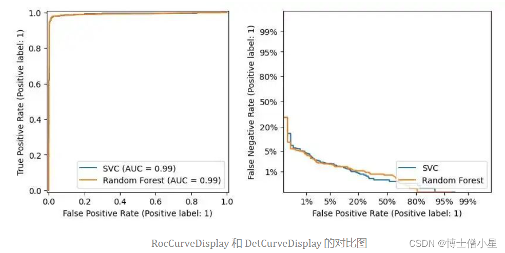
六、调整阈值
在数据不平衡的情况下,希望调整召回率和精确度。可以使用使用 metrics.PrecisionRecallDisplay 调整阈值
对于电子邮件欺诈,需要高精确度。
而对于疾病筛查,则需要高召回率来捕获更多病例。
那么可以调整阈值,但调整多少才合适呢?因此可以使用
metrics.PrecisionRecallDisplay来绘制相关图表。
from xgboost import XGBClassifier
from sklearn.datasets import load_wine
from sklearn.metrics import PrecisionRecallDisplay

wine = load_wine()
X, y = wine.data[wine.target<=1], wine.target[wine.target<=1]
X_train, X_test, y_train, y_test = train_test_split(X, y, test_size=0.3,
                                               stratify=y, random_state=42)

xgb_clf = XGBClassifier()
xgb_clf.fit(X_train, y_train)

PrecisionRecallDisplay.from_estimator(xgb_clf, X_test, y_test)
plt.show()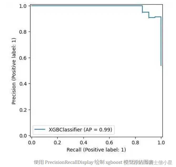
这表明可以按照 Scikit-learn 的设计绘制模型,就像这里的
xgboost。
七、回归模型评估
Scikit-learn 的
metrics.PredictionErrorDisplay绘制残差图可以帮助评估回归模型。
from sklearn.svm import SVR
from sklearn.metrics import PredictionErrorDisplay

rng = np.random.default_rng(42)
X = rng.random(size=(200, 2)) * 10
y = X[:, 0]**2 + 5 * X[:, 1] + 10 + rng.normal(loc=0.0, scale=0.1, size=(200,))

reg = make_pipeline(StandardScaler(), SVR(kernel='linear', C=10))
reg.fit(X, y)

fig, axes = plt.subplots(1, 2, figsize=(8, 4))
PredictionErrorDisplay.from_estimator(reg, X, y, ax=axes[0], kind="actual_vs_predicted")
PredictionErrorDisplay.from_estimator(reg, X, y, ax=axes[1], kind="residual_vs_predicted")
plt.show()
图表展示预测值与实际值的比较,左图适合线性回归。然而,并非所有数据都是完全线性的,因此,请参考右图。右图展示了实际值与预测值的差异,即残差图。残差图的香蕉形状暗示我们的数据可能不适合线性回归。考虑将核函数从"线性" 转换为 "rbf" ,残差图会更好。
reg = make_pipeline(StandardScaler(),
                    SVR(kernel='rbf', C=10))
八、绘制学习曲线
学习曲线主要研究模型的泛化效果和训练测试数据之间的差异或偏差。接下来,使用
model_selection.LearningCurveDisplay绘制学习曲线,并比较了决策树分类器和梯度提升分类器在不同训练数据下的表现。
from sklearn.tree import DecisionTreeClassifier
from sklearn.ensemble import GradientBoostingClassifier
from sklearn.model_selection import LearningCurveDisplay

X, y = make_classification(n_samples=1000, n_classes=2, n_features=10,
                           n_informative=2, n_redundant=0, n_repeated=0)

tree_clf = DecisionTreeClassifier(max_depth=3, random_state=42)
gb_clf = GradientBoostingClassifier(n_estimators=50, max_depth=3, tol=1e-3)

train_sizes = np.linspace(0.4, 1.0, 10)
fig, axes = plt.subplots(1, 2, figsize=(10, 4))
LearningCurveDisplay.from_estimator(tree_clf, X, y,
                                    train_sizes=train_sizes,
                                    ax=axes[0],
                                    scoring='accuracy')
axes[0].set_title('DecisionTreeClassifier')
LearningCurveDisplay.from_estimator(gb_clf, X, y,
                                    train_sizes=train_sizes,
                                    ax=axes[1],
                                    scoring='accuracy')
axes[1].set_title('GradientBoostingClassifier')
plt.show()
从图中可以看出,虽然基于树的
GradientBoostingClassifier在训练数据上保持了良好的准确性,但其在测试数据上的泛化能力与DecisionTreeClassifier相比并无明显优势。
九、可视化参数调整
为了改善泛化效果差的模型,可以尝试通过调整正则化参数来提高性能。传统的方法是使用 "GridSearchCV" 或 "Optuna" 等工具来实现模型调整,然而这些方法只能找出整体表现最佳的模型,且调整过程并不直观。如果需要调整特定参数以测试其对模型的影响,建议使用
model_selection.ValidationCurveDisplay来直观地观察模型在参数变化时的表现。
from sklearn.model_selection import ValidationCurveDisplay
from sklearn.linear_model import LogisticRegression

param_name, param_range = "C", np.logspace(-8, 3, 10)
lr_clf = LogisticRegression()

ValidationCurveDisplay.from_estimator(lr_clf, X, y,
                                      param_name=param_name,
                                      param_range=param_range,
                                      scoring='f1_weighted',
                                      cv=5, n_jobs=-1)
plt.show()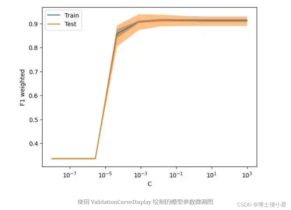
十、讨论
尝试过所有这些显示后,我必须承认一些遗憾:
最大的遗憾是这些 API 大多数缺乏详细的教程,这可能也是与 Scikit-learn 的详尽文档相比不为人知的原因。
这些应用程序接口散布在不同的软件包中,因此很难从一个地方引用它们。
代码仍然非常基础。通常需要将其与 Matplotlib 的 API 搭配使用才能完成工作。一个典型的例子是 "DecisionBoundaryDisplay",在绘制决策边界后,还需要使用 Matplotlib 来绘制数据分布。
它们很难扩展。除了一些验证参数的方法外,很难用工具或方法来简化模型的可视化过程;最终需要重写了很多东西。
这些 API 希望得到更多关注,并且随着版本升级,可视化 API 也能更易用。
在机器学习中,用可视化方式解释模型与训练模型同样重要。
本文介绍了当前版本 scikit-learn 中的各种绘图 API,利用这些 API,可以简化一些 Matplotlib 代码,缓解学习曲线,并简化模型评估过程。由于篇幅有限,未对每个 API 进行详细介绍。如果有兴趣,可以查看 [官方文档:https://scikit-learn.org/stable/visualizations.html?ref=dataleadsfuture.com] 了解更多详情。


![[Kubernetes] Rancher 2.7.5 部署 k8s](https://img-blog.csdnimg.cn/direct/22a22b8705fe4a738f1640dfa90bef46.png)